
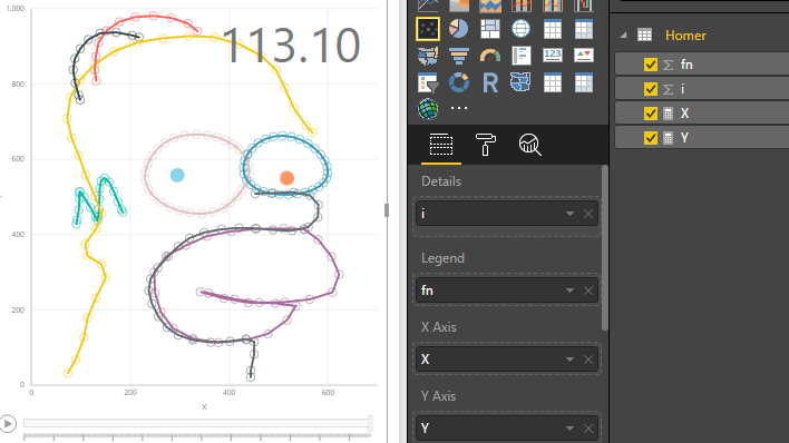
Recently I started exploring the limits of standard charts in Power BI and ended up drawing all sorts of mathematical functions. So I’ve decided to port a famous Homer Simpson-like curve to DAX for the fun of it and was impressed by the result.
As always, there is no magic involved, just the usual trio:
- Prepare some iterator ranges in M
- Add some curve functions in DAX
- Visualize it 😍
Depending on how you look at this, the final solution can be summarized into 65 LOC = 15 LOC of M + 2*25 LOC of DAX. But check out the curves on those lines.
The M code
The Power Query code necessary for this doodle generates some specific ranges for drawing various parts of the cartoon figure. For convenience, all of them are expressed in units of π.
| let | |
| //generate a range between [start] and [end] in number of [steps] with a category descriptor | |
| range = (category,steps,start,end)=>List.Accumulate({1..steps},{{category,start}},(s,c)=>s&{{category,start+(c/steps)*(end-start)}}), | |
| //shortcut | |
| pi = Number.PI | |
| //stiching multiple ranges into a an iterator table | |
| in #table(type table[#"fn"=number,#"i"=number], | |
| range(0,20,35*pi,36*pi)& | |
| range(1,10,31*pi,32*pi)& | |
| range(2,10,27*pi,28*pi)& | |
| range(3,30,23*pi,24*pi)& | |
| range(4,30,19*pi,20*pi)& | |
| range(5,30,15*pi,17*pi)& | |
| range(6,30,11*pi,13*pi)& | |
| range(7,30,7*pi,9*pi)& | |
| range(8,30,3*pi,5*pi)& | |
| range(9,30,1*pi,3*pi)) |
The DAX code
The DAX code is broken down into 2 measure for X and Y coordinates. Each measure performs two steps:
- Define a collection of 10 heavily trigonometric functions (fn[index])
- Map the curve function fn[index] to a category fn which corresponds to a drawing range iterator
X coordinates measure
| X = | |
| VAR t = LASTNONBLANK(Homer[i],1) | |
| VAR fnX = LASTNONBLANK(Homer[fn],1) | |
| VAR fn0 = (-11/8*sin(17/11 - 8*t) - 3/4*sin(11/7 - 6*t) - 9/10*sin(17/11 - 5*t) + 349/9*sin(t + 11/7) + 17/12*sin(2*t + 8/5) + 288/41*sin(3*t + 8/5) + 69/10*sin(4*t + 8/5) + 8/5*sin(7*t + 13/8) + 4/7*sin(9*t + 28/17) + 4/7*sin(10*t + 19/11) + 1051/8) | |
| VAR fn1 = (-3/4*sin(11/7 - 5*t) - 54*sin(11/7 - t) + 237/8*sin(2*t + 11/7) + 52/11*sin(3*t + 33/7) + 38/9*sin(4*t + 11/7) + 249/2) | |
| VAR fn2 = (-16/9*sin(14/9 - 5*t) - 5/2*sin(14/9 - 3*t) + 781/8*sin(t + 33/7) + 291/11*sin(2*t + 11/7) + 23/7*sin(4*t + 11/7) + 18/19*sin(6*t + 11/7) + 2/5*sin(7*t + 61/13) + 24/23*sin(8*t + 14/9) + 1/27*sin(9*t + 5/11) + 4/11*sin(10*t + 11/7) + 1/75*sin(11*t + 5/8) + 1411/7) | |
| VAR fn3 = (-7/11*sin(13/10 - 13*t) + 3003/16*sin(t + 33/7) + 612/5*sin(2*t + 11/7) + 542/11*sin(3*t + 47/10) + 137/7*sin(4*t + 51/11) + 53/7*sin(5*t + 17/11) + 23/12*sin(6*t + 41/9) + 94/11*sin(7*t + 51/11) + 81/11*sin(8*t + 41/9) + 53/12*sin(9*t + 23/5) + 73/21*sin(10*t + 13/9) + 15/7*sin(11*t + 6/5) + 37/7*sin(12*t + 7/5) + 5/9*sin(14*t + 27/7) + 36/7*sin(15*t + 9/2) + 68/23*sin(16*t + 48/11) + 14/9*sin(17*t + 32/7) + 1999/9) | |
| VAR fn4 = (1692/19*sin(t + 29/19) + 522/5*sin(2*t + 16/11) + 767/12*sin(3*t + 59/13) + 256/11*sin(4*t + 31/7) + 101/5*sin(5*t + 48/11) + 163/8*sin(6*t + 43/10) + 74/11*sin(7*t + 49/12) + 35/4*sin(8*t + 41/10) + 22/15*sin(9*t + 29/14) + 43/10*sin(10*t + 4) + 16/7*sin(11*t + 6/5) + 11/21*sin(12*t + 55/14) + 3/4*sin(13*t + 37/10) + 13/10*sin(14*t + 27/7) + 2383/6) | |
| VAR fn5 = (-1/9*sin(7/5 - 10*t) - 2/9*sin(11/9 - 6*t) + 20/11*sin(t + 16/15) + 7/13*sin(2*t + 15/4) + 56/13*sin(3*t + 25/9) + 1/6*sin(4*t + 56/15) + 5/16*sin(5*t + 19/8) + 2/5*sin(7*t + 5/16) + 5/12*sin(8*t + 17/5) + 1/4*sin(9*t + 3) + 1181/4) | |
| VAR fn6 = (-1/6*sin(8/11 - 5*t) + 5/8*sin(t + 6/5) + 13/5*sin(2*t + 45/14) + 10/3*sin(3*t + 7/2) + 13/10*sin(4*t + 24/25) + 1/6*sin(6*t + 9/5) + 1/4*sin(7*t + 37/13) + 1/8*sin(8*t + 13/4) + 1/9*sin(9*t + 7/9) + 2/9*sin(10*t + 63/25) + 1/10*sin(11*t + 1/9) + 4137/8) | |
| VAR fn7 = (-17/13*sin(6/5 - 12*t) - 15/7*sin(25/26 - 11*t) - 13/7*sin(3/14 - 10*t) - 25/7*sin(9/13 - 6*t) - 329/3*sin(8/17 - t) + 871/8*sin(2*t + 2) + 513/14*sin(3*t + 5/4) + 110/9*sin(4*t + 3/8) + 43/8*sin(5*t + 1/5) + 43/13*sin(7*t + 42/11) + 49/16*sin(8*t + 11/13) + 11/5*sin(9*t + 2/7) + 5/7*sin(13*t + 42/13) + 1729/4) | |
| VAR fn8 = (427/5*sin(t + 91/45) + 3/11*sin(2*t + 7/2) + 5656/11) | |
| VAR fn9 = (-10/9*sin(7/10 - 4*t) - 7/13*sin(5/6 - 3*t) - 732/7*sin(4/7 - t) + 63/31*sin(2*t + 1/47) + 27/16*sin(5*t + 11/4) + 3700/11) | |
| RETURN | |
| SWITCH(TRUE(), | |
| fnX=0,fn0, | |
| fnX=1,fn1, | |
| fnX=2,fn2, | |
| fnX=3,fn3, | |
| fnX=4,fn4, | |
| fnX=5,fn5, | |
| fnX=6,fn6, | |
| fnX=7,fn7, | |
| fnX=8,fn8, | |
| fnX=9,fn9, | |
| BLANK()) |
Y coordinates measure
| Y = | |
| VAR t = LASTNONBLANK(Homer[i],1) | |
| VAR fnX = LASTNONBLANK(Homer[fn],1) | |
| VAR fn0 = (-4/11*sin(7/5 - 10*t) - 11/16*sin(14/13 - 7*t) - 481/11*sin(17/11 - 4*t) - 78/7*sin(26/17 - 3*t) + 219/11*sin(t + 11/7) + 15/7*sin(2*t + 18/11) + 69/11*sin(5*t + 11/7) + 31/12*sin(6*t + 47/10) + 5/8*sin(8*t + 19/12) + 10/9*sin(9*t + 17/11) + 5365/11) | |
| VAR fn1 = (-75/13*sin(14/9 - 4*t) - 132/5*sin(11/7 - 2*t) - 83*sin(11/7 - t) + 1/7*sin(3*t + 47/10) + 1/8*sin(5*t + 14/11) + 18332/21) | |
| VAR fn2 = (191/3*sin(t + 33/7) + 364/9*sin(2*t + 33/7) + 43/22*sin(3*t + 14/3) + 158/21*sin(4*t + 33/7) + 1/4*sin(5*t + 74/17) + 121/30*sin(6*t + 47/10) + 1/9*sin(7*t + 17/6) + 25/11*sin(8*t + 61/13) + 1/6*sin(9*t + 40/9) + 7/6*sin(10*t + 47/10) + 1/14*sin(11*t + 55/28) + 7435/8) | |
| VAR fn3 = (-4/7*sin(14/9 - 13*t) + 2839/8*sin(t + 47/10) + 893/6*sin(2*t + 61/13) + 526/11*sin(3*t + 8/5) + 802/15*sin(4*t + 47/10) + 181/36*sin(5*t + 13/3) + 2089/87*sin(6*t + 14/3) + 29/8*sin(7*t + 69/16) + 125/12*sin(8*t + 47/10) + 4/5*sin(9*t + 53/12) + 93/47*sin(10*t + 61/13) + 3/10*sin(11*t + 9/7) + 13/5*sin(12*t + 14/3) + 41/21*sin(14*t + 22/5) + 4/5*sin(15*t + 22/5) + 14/5*sin(16*t + 50/11) + 17/7*sin(17*t + 40/9) + 4180/7) | |
| VAR fn4 = (-7/4*sin(8/11 - 14*t) - 37/13*sin(3/2 - 12*t) + 2345/11*sin(t + 32/21) + 632/23*sin(2*t + 14/3) + 29/6*sin(3*t + 31/21) + 245/11*sin(4*t + 5/4) + 193/16*sin(5*t + 7/5) + 19/2*sin(6*t + 32/7) + 19/5*sin(7*t + 17/9) + 334/23*sin(8*t + 35/8) + 11/3*sin(9*t + 21/11) + 106/15*sin(10*t + 22/5) + 52/15*sin(11*t + 19/12) + 7/2*sin(13*t + 16/13) + 12506/41) | |
| VAR fn5 = (-3/7*sin(1/10 - 9*t) - 1/8*sin(5/14 - 5*t) - 9/8*sin(26/17 - 2*t) + 18/7*sin(t + 14/11) + 249/50*sin(3*t + 37/8) + 3/13*sin(4*t + 19/9) + 2/5*sin(6*t + 65/16) + 9/17*sin(7*t + 1/4) + 5/16*sin(8*t + 44/13) + 2/9*sin(10*t + 29/10) + 6689/12) | |
| VAR fn6 = (-1/27*sin(1 - 11*t) - 1/6*sin(4/11 - 10*t) - 1/5*sin(2/11 - 9*t) - 7/20*sin(1/2 - 5*t) - 51/14*sin(29/28 - 3*t) + 23/7*sin(t + 18/5) + 25/9*sin(2*t + 53/12) + 3/2*sin(4*t + 41/15) + 1/5*sin(6*t + 36/11) + 1/12*sin(7*t + 14/3) + 3/10*sin(8*t + 19/9) + 3845/7) | |
| VAR fn7 = (-8/7*sin(1/3 - 13*t) - 9/13*sin(4/5 - 11*t) - 32/19*sin(17/12 - 9*t) - 11/6*sin(9/13 - 8*t) - 169/15*sin(8/17 - 3*t) + 917/8*sin(t + 55/12) + 669/10*sin(2*t + 4/13) + 122/11*sin(4*t + 49/24) + 31/9*sin(5*t + 1/8) + 25/9*sin(6*t + 6/7) + 43/10*sin(7*t + 1/21) + 18/19*sin(10*t + 9/13) + 2/9*sin(12*t + 31/15) + 1309/5) | |
| VAR fn8 = (-267/38*sin(3/10 - 2*t) + 625/8*sin(t + 62/17) + 8083/14) | |
| VAR fn9 = (1370/13*sin(t + 25/6) + 41/21*sin(2*t + 205/51) + 11/16*sin(3*t + 8/13) + 9/13*sin(4*t + 26/9) + 6/5*sin(5*t + 11/14) + 2251/4) | |
| RETURN | |
| SWITCH(TRUE(), | |
| fnX=0,fn0, | |
| fnX=1,fn1, | |
| fnX=2,fn2, | |
| fnX=3,fn3, | |
| fnX=4,fn4, | |
| fnX=5,fn5, | |
| fnX=6,fn6, | |
| fnX=7,fn7, | |
| fnX=8,fn8, | |
| fnX=9,fn9, | |
| BLANK()) |
The visual
To build the visualization:
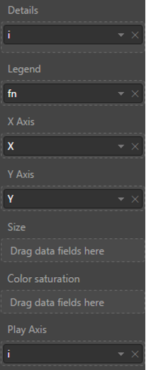
- Select the standard Scattered Chart.
- Add column i to Details and Play Axis.
- Add fn to the Legend.
And to finish all off, map X to X Axis and Y to Y axis — DOH!
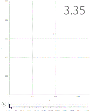
Select all of the fn ids from the charts’ Legend and press play.
The origin
For the curious minds, the functions above were taken from WolframAlpha. In addition, their scientists have written a series of blog posts in which they describe the steps required for generating various curves in minute detail. Start with:
Making Formulas… for Everything—From Pi to the Pink Panther to Sir Isaac Newton
It would be an understatement to I say that everything boils down to a Fast Fourier Transform — but it does 🙂
And finally — here is the original Homer Simpson-like curve:

that’s funny : ) how should I paste the m code into power query? should I convert it to list or table? should I rename it to homer or what? I couldnt create the pbix file.
LikeLike
You’re on the right path.
Copy the m code into power query editor. Make sure to replace all the wrapper code there. Rename the query to “Homer”. And add the DAX code as measure to this Homer table. After replicating the setup as in the scatter chart you should see the Homer’s dotted figure. If you want to replicate the animation, select all of the fn values from the legend (values 0..9), now slide the play axis and you should see the figure as being drawn.
LikeLike
Hi there! Thanks for this article, that’s really awesome!
But i can’t replicate the animation with lines, just dots which moving. Could you please write about lines with more detailes?
LikeLike